It All Starts With Noise!

Avada Kedavra!

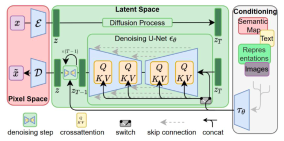
Don’t worry, this isn’t the Dark Arts class ;). This high-level architecture diagram of a Stable Diffusion model may look terrifying, but it’s going to make sense in just a few minutes.

In this blog, we will understand a diffusion model from scratch. Here we will discuss the various elements that make a stable diffusion model.

Flow Matching

In physics, “flow” describes how particles move over time, just like tracing ink diffusing in water. Flow matching in diffusion models draws inspiration from this concept.

In ML terms:

Forward flow: Clean data → progressively noisier data (like adding Gaussian noise). Reverse flow: Noise → clean data (like denoising step by step).

A vector field describes the direction you should move in to go from one distribution to another. So, flow matching means learning a vector field (e.g., gradients or velocities) to “reverse” the noise trajectory and recover the data. Learn more

In diffusion models:

Forward flow is known (we define the noise schedule). Reverse flow is learned using neural networks (where U-Net comes in!)

---

Diffusion

Stable Diffusion belongs to a class of deep learning models called diffusion models. These are generative models, which means they’re designed to generate new data similar to what they saw during training. In the case of Stable Diffusion, this data is images.

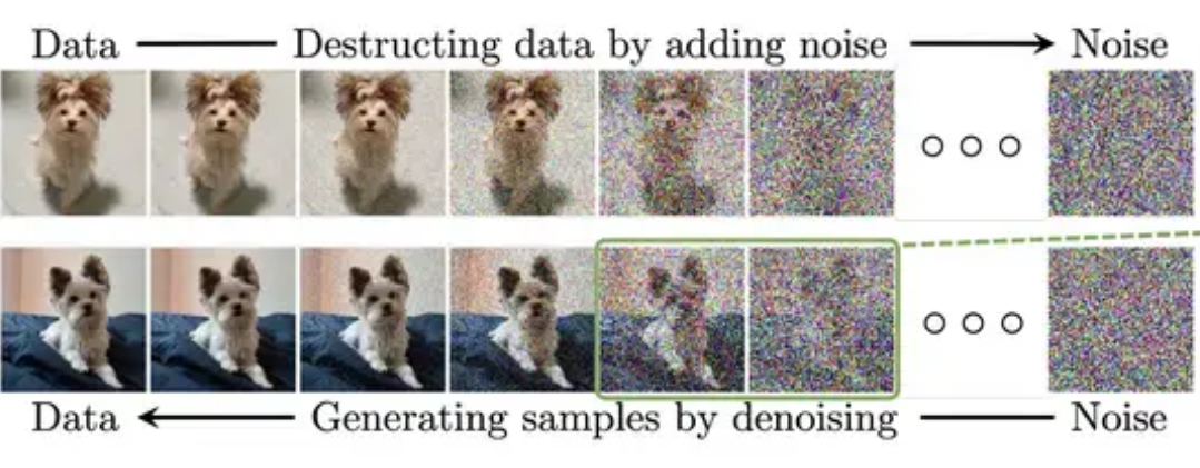
Forward Diffusion

The forward process is all about adding noise to an image, step-by-step, until the image becomes like random noise.

Imagine we trained the model only on images of cats and dogs. Initially, these images form two distinct clusters. As we apply forward diffusion, we add noise over many steps, and eventually, all images (cat or dog) end up looking like pure noise.

Reverse Diffusion

What if we could revert the noise process? Starting from noise, what if we could recover the original image?

That’s exactly what diffusion models do: they learn how to reverse the diffusion process. Starting with random noise, they denoise step-by-step until a realistic image emerges.

Training the Noise Predictor and the Reverse Process (Noise to Nice)

So how do we train a model to do this reverse process?

We teach a neural network to predict the noise that was added during the forward process. In Stable Diffusion, this noise predictor is a U-Net model.

Steps:

1. Take a clean image.
2. Generate some random noise.
3. Add that noise to the image (forward diffusion).
4. Train the U-Net to predict the noise that was added.

During generation:

1. Start with pure noise.
2. Use the trained U-Net to predict the noise.
3. Subtract the predicted noise.
4. Repeat the process many times.

Initially, this process is unconditional. With conditioning (e.g., text prompts), we can guide the output.

---

Latent Diffusion Model: Making It Fast

One of the biggest challenges with earlier diffusion models was speed. They operated directly on pixel space itself , and it was expensive.

Stable Diffusion solves this by using a latent diffusion model ;it doesn’t operate in pixel space but in a smaller latent space (about 48× smaller), making everything faster and more efficient.

Architecture Overview of SD :

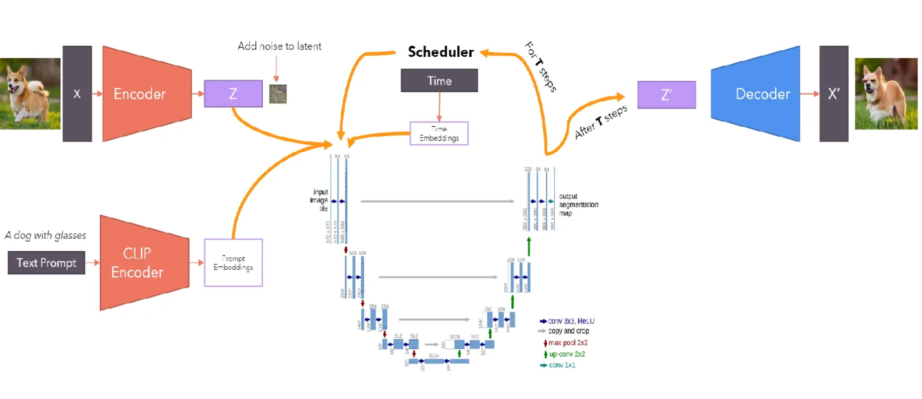
Here’s what the architecture looks like:

• VAE for latent space encoding/decoding
• Optional text encoder for conditional generation
• U-Net for noise prediction

---

Wait! if you’re new to concepts like VAEs, CLIP, or self-attention, just go through them briefly, but feel free to continue regardless;

Variational Autoencoder (VAE)

Compression to latent space is done using a Variational Autoencoder (VAE).

A VAE has:

1. Encoder – Compresses image into latent space
2. Decoder – Reconstructs the image

In Stable Diffusion, all forward and reverse diffusion happens in this latent space, not pixel space. So , When generating images, the diffusion process operates in the latent space, not directly on the image pixels. Also, after the model denoises the latent, the decoder part of the VAE reconstructs the final image from this latent.

Clip Encoder

CLIP (Contrastive Language–Image Pre-training) is a model that learns to connect images and text. It creates similar embeddings (encodings) for an image and its matching caption, so they can be compared directly.

The image below shows how CLIP compares images and text. The text and image embeddings are compared using dot products. A higher dot product means a stronger match.

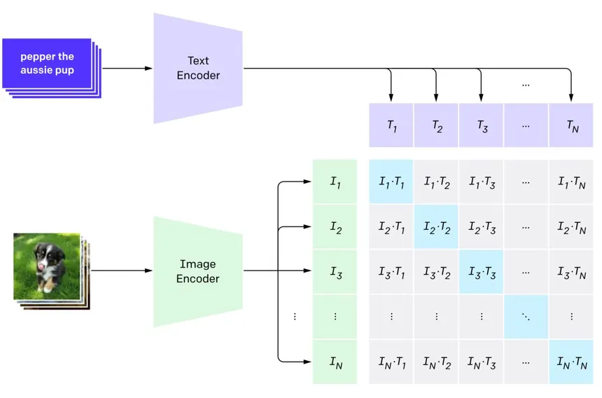
You could also say:

CLIP is a model that understands images and text together. It learns to match a picture with the right caption by putting them close in a shared space, making it useful for tasks like image search or classification using text.

If you are curious you can read more about CLIP in this article.

Scheduler

A scheduler is a key component in diffusion models. At every timestamp, it controls how noise is added during the forward diffusion process and also guides how noise is removed during the reverse denoising process. It also determine the pace and structure of the entire diffusion process. For ex, I have a complete noise image and during the early iterations I remove most of the predicted noise. But as the time passes, I start decreasing the strength and remove less noise than what was actuallly predicted in order to not loose important info. Different schedulers (linear, cosine, DDIM, etc.) use different noise strategies. The choice of scheduler can affect image quality, speed, and stability.

---

The DDPM Process

Now let’s understand the actual math that powers forward and reverse diffusion.

Forward Diffusion Process

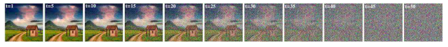
In the forward diffusion step, we gradually add noise to the image or data over multiple steps until it becomes close to pure Gaussian noise. This process is repeated over a fixed number of timesteps, with a small amount of Gaussian noise added at each step. As the number of steps increases, the image becomes more noisy and over a lot of steps nearing to pure Gaussian noise. This sequence can be visualized as follows:

Each forward step is:

$$q(x_t \mid x_{t-1}) = \mathcal{N}(x_t; \sqrt{1 - \beta_t} \, x_{t-1}, \beta_t \mathbf{I})$$

Where:

• $q$ is the forward process distribution.
• $x_t$ is the noisy data at timestep $t$.
• $x_{t-1}$ is the data from the previous timestep.
• $\mathcal{N}$ denotes a normal (Gaussian) distribution.
• The mean is $\sqrt{1 - \beta_t} \, x_{t-1}$.
• The variance is $\beta_t \mathbf{I}$, where $\mathbf{I}$ is the identity matrix.

The above equation just suggests us that we are adding more noise to our data as and when we proceed to the next step. We are just changing the mean and variance of the distribution and making it converge to pure Gaussian Noise.

$\beta_t$ is something called schedule and decides what amount of noise is to be added in each step. Researchers from OpenAI designed their own schedule and called it the cosine schedule. This is produced by the scheduler discussed above.

Now we will represent $x_t$ using $x_0$ instead of $x_{t-1}$. This can be done by representing $x_{t-1}$ in terms of $x_0$ and so on. For $t$ steps, it can be represented as:

$$q_t(q_{t-1}(q_{t-2}(\dots q_1(x_0))))$$

We see that only the mean depends on the previous step and $\beta_t \mathbf{I}$ is already known for each $t$.

To simplify the math, let us say:

$$\alpha_t = 1 - \beta_t \qquad \bar{\alpha}_t := \prod_{s=1}^t \alpha_s$$

So now we can write

$$q(x_1 \mid x_0) = \mathcal{N}(x_1; \sqrt{\alpha_1} \, x_0, (1 - \alpha_1) \mathbf{I})$$

As the process continues, the mean $\mu_t$ evolves as:

$$\mu_t = \sqrt{\alpha_t \alpha_{t-1}} \, x_{t-2} = \dots = \sqrt{\bar{\alpha}_t} \, x_0$$

Now we can finally write $x_t$ directly as a function of $x_0$ as follows:

$$q(x_t \mid x_0) = \mathcal{N}(x_t; \sqrt{\bar{\alpha}_t} \, x_0, (1 - \bar{\alpha}_t) \mathbf{I})$$

or,

$$q(x_t \mid x_0) = \sqrt{\bar{\alpha}_t} \, x_0 + \sqrt{1 - \bar{\alpha}_t} \cdot \epsilon, \quad \epsilon \sim \mathcal{N}(0, \mathbf{I})$$

---

Reverse Diffusion

As I have said multiple times, reverse diffusion means that we are removing the noise and creating a new image. But instead of removing the noise, this predicts the noise that has to be removed and then subtracts it from the noisy image to get a clearer image. This step is also repeated multiple times until we get a good quality image.

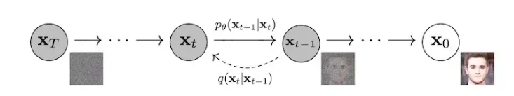
Now because direct computation of $q(x_{t-1} \mid x_t)$ is difficult, we learn a model $p_\theta$ to approximate it.

The reverse process is defined as:

$$p_\theta(x_{0:T}) = p(x_T) \prod_{t=1}^{T} p_\theta(x_{t-1} \mid x_t)$$

with each transition modeled as:

$$p_\theta(x_{t-1} \mid x_t) = \mathcal{N}(x_{t-1}; \mu_\theta(x_t, t), \Sigma_\theta(x_t, t))$$

Even though this equation looks deadly, lets break it down to understand it easily. Now in reverse diffusion we want to have $x_{t-1}$ from $x_t$, this gives us the LHS of the equation. Now it can be defined as a Gaussian distribution, with mean $\mu_\theta(x_t, t)$ and variance $\Sigma_\theta(x_t, t))$. This just suggests that the mean and the variance is just a function of $x_t$ and $t$.

To train this model, we use the ELBO (Evidence Lower Bound) or the Jensen’s inequality, which helps us optimize a lower bound on the data likelihood:

$$L_{\text{VLB}} = \mathbb{E}_{q(\mathbf{x}_{0:T})} \left[ \log \frac{q(\mathbf{x}_{1:T} \mid \mathbf{x}_0)}{p_\theta(\mathbf{x}_{0:T})} \right] \geq -\mathbb{E}_{q(\mathbf{x}_0)} \log p_\theta(\mathbf{x}_0)$$

After a lot of mathematical derivation (which can be found here) we get,

$$\mu_\theta(x_t, t) = \frac{1}{\sqrt{\alpha_t}} \left( x_t - \frac{1 - \bar{\alpha}_t}{\sqrt{1 - \alpha_t}} \epsilon_\theta(x_t, t) \right)$$

Using this mean, the final equation becomes:

$$x_{t-1} = \frac{1}{\sqrt{\alpha_t}} \left( x_t - \frac{1 - \bar{\alpha}_t}{\sqrt{1 - \bar{\alpha}_t}} \beta_t \epsilon_\theta(x_t, t) \right) + \sqrt{\beta_t} \cdot \epsilon$$

where $\epsilon \sim \mathcal{N}(0, I)$ is Gaussian noise. At the final denoising step (i.e., $t = 1$), we do not add the noise term $\sqrt{\beta_t} \cdot \epsilon$, because we want the clean sample: $x_0 = \mu_\theta(x_1, 1)$

---

U-Net

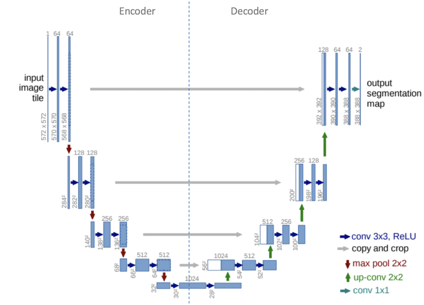
Now, coming to U-Net ,the special neural network we use for denoising. It has an encoder-decoder structure with skip connections that preserve spatial information.

The encoder (downsampling path) reduces spatial resolution while increasing feature depth using ResNet blocks and downsampling layers. The decoder (upsampling path) gradually restores resolution using upsampling and ResNet blocks, combining features from the encoder via skip connections.

Timestep information is encoded using sinusoidal positional embeddings, while text prompts are encoded using the CLIP model. These embeddings are passed into the ResNet blocks to guide the denoising process. Then , attention layers are added in deeper blocks to capture long-range dependencies and also go accord to the prompt.

The output of U-Net is the predicted noise for the current timestep, which is used to iteratively reconstruct the image.

Before looking at the individual architecture blocks, it’s important to understand how the U-Net receives information about the timestep and prompt.

Although it may appear that the U-Net only processes a noisy image, it also receives two conditioning inputs:

• A timestep embedding that encodes the current diffusion step using sinusoidal positional encoding (similar to Transformer encodings).
• A prompt embedding (ex., from CLIP or a class label encoder), which provides conditioning information for text-to-image generation or class-conditional generation.

These embeddings are summed and passed into each ResNet block inside the U-Net.

Downsample Block

In downsampling process. spatial resolution is reduced. Each downsample block:

• Receives feature maps from the previous layer.
• Uses a downsampling operation (e.g., max pooling) to reduce resolution.
• Applies two ResNet blocks, each conditioned on the timestep and prompt embeddings (projected and added to the feature map).
• In some blocks, self-attention layers are used to allow spatial positions to interact globally.

Self-Attention Block

Attention blocks replace some ResNet blocks in deeper layers. The input is reshaped from 2D to a sequence of tokens for Multi-Head Attention (MHA). For example, a feature map of shape (128, 32, 32) is reshaped to (1024, 128) and passed through:

• LayerNorm
• Attention (Q, K, V from the same input)
• A feedforward network with skip connections
• The output is reshaped back to (128, 32, 32)

This enables the network to model long-range dependencies and better align image features with text tokens.

Upsample Block

The upsampling path increases resolution and reconstructs spatial detail. Each upsample block:

• Upsamples the feature map.
• Concatenates it with the corresponding feature map from the encoder (via skip connections).
• Passes the result through two ResNet blocks.
• Like in the encoder, the timestep ,plus prompt embedding is projected and added.

The final convolutional layer reduces the number of channels back to the original latent size (e.g., from (64, 64, 64) to (4, 64, 64)), producing the predicted noise at that timestep.

The U-Net in Stable Diffusion is thus a conditional denoising network that receives a noisy latent image, timestep embedding, and prompt embedding, and predicts the noise component to be removed at that step of the reverse diffusion process.

---

Conclusion

We’ve seen all the components of the architecture of Stable Diffusion . Summarizing all this: we have an input image and a prompt, first using the VAE encoder we encode a higher dimensional image into a lower dimensional latent space where we apply diffusion .

One of the important categories of diffusion is DDPM wherein we had a gaussian noise at each timestep and then , using U-Net ,we predicted the noise and removed a part of it using the dynamic scheduler iteratively until we obtained our desired/ clean image..

Also, in the U-Net step, we used attention between the image and embeddings of the prompt (generated by oneee and onlyy CLIP). Now, from the latent space , we go to pixel space by riding the decoder and hence we get the image.

Understanding each component is key to appreciating how the model works and what makes it both efficient and powerful.

---

Thanks for reading. If you want to dive deeper, explore the math behind diffusion models, experiment with open-source implementations, or try generating your own images with Hugging Face Spaces or Stable Diffusion APIs.